Multi-Core Acceleration and Embedded Optimization of Rear Vehicle Detection Algorithms Denso Camera Mirror Replacement, algorithm porting and optimization

Multi-Core Acceleration and Embedded Optimization of Rear Vehicle Detection Algorithms Denso Camera Mirror Replacement, algorithm porting and optimization


Short introduction

Camera mirror replacement system (CMRS), which are now replacing as many as six mirrors on trucks, may require two cameras on the driver’s side and two cameras on the passenger side, rendering the video streams to create a very wide view. The main idea behind this algorithm is to detect a car approaching from behind and alert the driver in case of potential collision. The algorithm is created by DENSO for PCs. Here we will focus on porting and optimization of one of such algorithms for the embedded target platform.

Target platform and SoC overview

As the algorithm is initially created for the PCs, the main goal is to do the porting and optimization for the ALPHA embedded platform. The ALPHA board consists of three interconnected TDA2x SoCs. One of those will be used as a target SoC in the process of porting and optimization. The platform is depicted in Figure 1.

Denso Camera Mirror Replacement - Target platform and SoC overview

Figure 1. – ALPHA board

The selected TDA2x SoC (colored in red) has the following resources.

2xDSP C66x cores:

  • SIMD Floating point
  • Up to eight instructions executed per cycle

2x ARM Cortex-A15 cores:

  • SIMD Floating point
  • Good support for software cache prefetching

4x Embedded Vision Engine cores:

  • Integer SIMD instructions
  • 16 16×16 multipliers
  • 768 bits/cycle memory access
  • Enhanced DMA

2x ARM Cortex-M4 2x cores:

  • dedicated to be a controlling processors, not data processing units
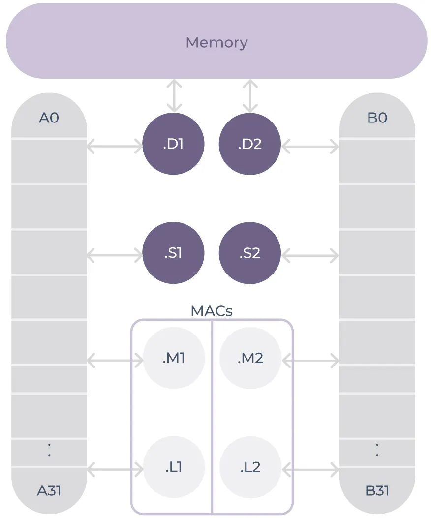
RM Cortex-M4 2x cores

Project overview

The starting point of the acquired algorithm was a single frame car detection PC application able to process a single frame at ~40ms. It was able to do car detection and car tracking working at ~25FPS in release mode with more demanding PC configuration. The algorithm itself could be split into four parts:

  1. Input frame processing and conversion from YUV422 to grayscale image
  2. Histogram of oriented gradients integral image computation
  3. Cascade classifier of predefined rectangle regions
  4. Kalman filter and YUV422 byte reordering

Initial step was porting of this single frame application from the PC to the target SoC. This was done in four, not so straight-forward, steps:

  1. Removal of unused code
  2. Creation of adequate VisionSDK algorithm plugins and use case
  3. Implementation of stdio capabilities for VisionSDK on Alpha board in order to read detection configuration
  4. Verification of detection results

Several main challenges in this stage of the project were to remove polymorphism in the code base as it would be hard to find the bottlenecks and do the optimization afterwards and to remove dependency on the textual configuration files as reading from the SD card was not possible on each SoC of the platform.

The first iteration yielded a ported version to the A15 core only. For the sake of simplicity and easier comparison of the results between the PC version (which is used as a ground-through reference) and ported and, later on, optimized version – the ethernet connection is used instead of cameras. Even though the hardware usage was modest, the algorithm porting was successful. Anyhow, using only A15 for both network transfer and all stages of the algorithm – the bottleneck was obvious.

For code optimization the target was processing only one image 1280×800 @ 30FPS. Several values to monitor have been defined to verify performance of the code (Boundary Boxes, Confidence, Distance and Speed) with the PC version as a ground-truth reference.

The first iteration of the optimization was to offload the A15 core with classification part of the algorithm. Both DSPs were used and the use case in the end looked like on Figure 2 (Use case after the first iteration of optimization).
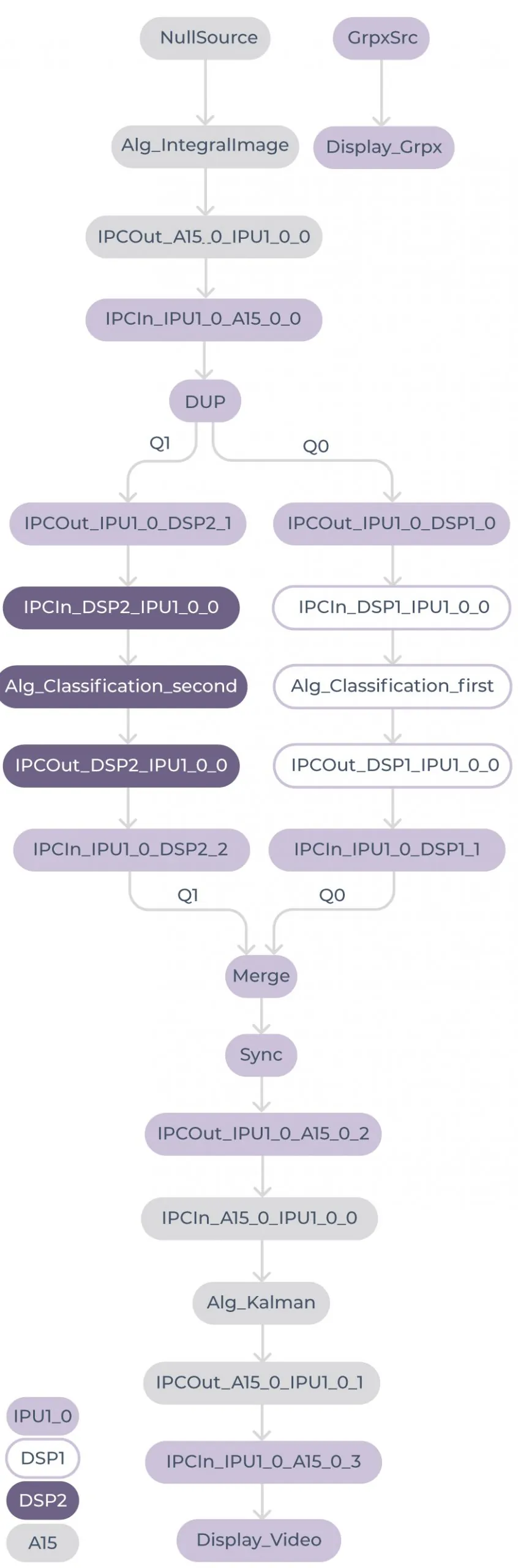
VisionSDK on Alpha board - after the first iteration of optimization
The observations after first decomposition were:

  • High demand on A15 due to network transfer
  • Poor classification performance of DSPs
    • Slow memory accesses
    • High performance penalty for each floating point division
    • Almost no parallelization on instructions level
  • Low demand of Kalman filter plugin
    • Kalman filter calculations – a few milliseconds
    • Conversion of YUV422 bytes order – a bit more
  • Good integral image algorithm plugin on A15
    • Full NEON vectorization
    • Running at ~54ms
  • Hardware still not utilized as it should be

To address the problems the approach was to:

  • Reduce unnecessary load on A15 core
    • Transferring whole video to board and then streaming it from memory (this is realistic scenario cause real data would come from cameras)
  • Rearrange the algorithm plugins
    • Splitting classification on A15 and one DSP
      • The majority of hypotheses processed on A15
      • Second DSP used to reduce load on A15
      • Calculation time ~105ms
    • Integral image moved to first DSP
      • Initially poor performance, calculation took around ~184ms
    • Kalman filter and YUV422 bytes reordering moved to M4
      • Calculation time ~54ms

By doing that we have got to the second iteration of the decomposition and therefore a better hardware utilization depicted on Figure 3. This was a starting point for the optimizations. For the classification part of the algorithm, the general optimization was to focus on the following:

  1. As hypotheses are generated at startup and classification of one ROI doesn’t affect the other, we can split hypotheses and process them in parallel!
  2. Tabulating repetitive calculations
  3. Analysis and removal of unnecessary calculations
  4. Branching removal
  5. Switching from division to multiplication with reciprocal value where possible
  6. Usage of intrinsics

After an analysis, we identified stages 1, 2 and 5 as the most critical stages in the classification. To address those, we precalculated the lookup tables. For stage 1, we figured out that for each ROI we can pre-calculate and store 4 pointer offsets to integral image and reciprocal value of area because everything is known at the time when ROIs are generated, which is in the initialization phase before any processing. For stage 2 we used a similar technique to store scaled rectangles for each sub stage of stage 2. Using the same trick as for stage 1 is not a good approach since we have 3 sub stages which would result in 3x bigger lookup table and that would be stressful on memory.
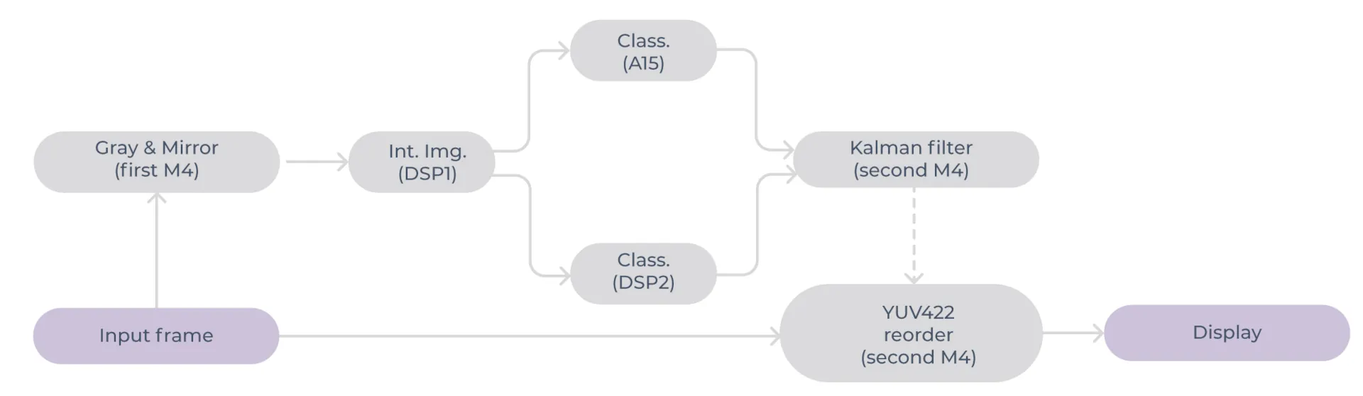
Second iteration of optimization

Figure 3. – Second iteration of optimization

For the A15 core specific optimization techniques we focused on:

  • Usage of vectorized SIMD instructions (ARM NEON)
  • Operating on 128 bit registers (e.g. 4 single precision floating point numbers, 16 unsigned bytes etc.)
  • Using ARM NEON
  • Using lookup tables helped but effect wasn’t as we expected due to newly induced cache misses
  • Exploiting cache prefetch instruction in combination with lookup table – use lookup table to prefetch data that will be needed shortly

For the DSP specific optimization techniques we focused on:

  • Replacing division with fast reciprocal value intrinsic + multiplication
    • To achieve the same precision 2 additional iteration of Newton-Raphson method were applied
  • Using DSP specific SIMD intrinsics
  • Unraveling data dependencies

Regarding the another CPU-heavy part of the algorithm – integral image – we have used the following techniques:

  • Heavy usage of DSP intrinsics
  • Preventing cache misses by removing lookup table for magnitude and bins
  • If dx is positive simple comparison between dx and absolute value of dy will tell us bin value
  • If dx is negative we can again compare absolute value of dx and absolute value of dy and get bin value
  • To remove branching we observed that we can calculate the bin value by comparing abs(dx) and abs(dy) and then doing the following correction if dx is negative:
    • Use abs(dx+1) instead of abs(dx)
    • XOR bin value with 3 (1 ^ 3 = 2, 0 ^ 3 = 3, this follows symmetry of distribution of bins)
  • Replacing expensive floating point calculation with integer multiplication and shifting

Final results

After this time-boxed optimization, we have got the algorithm on the target platform that is processing video at ~12 FPS. Average times for each part:

  • Gray & Mirror ~75ms
  • Integral image of HoG ~72ms
  • Classifier A15 ~60ms
  • Classifier DSP ~65ms
  • Kalman filter ~4ms
  • YUV 422 reorder ~50ms

Conclusion and possible improvement
Afterall, we have shown that the porting and optimization of the PC algorithm is possible. Of course there is always room for improvement. Here is the list for possible improvements. If we had more time we would definitely love to see the results of the following:

  • Use non-blocking DMA transfer to SRAM memory
    • Overlapping memory transfer and processing
    • Overhead for first block only
  • Reconfiguring DSP memory
    • 128KB L2 data cache
    • 128KB SRAM -> utilize non-blocking DMA!
  • Move algorithm some plugins to EVE (free DSP in process)
    • Great performance expected for integral image and YUV 422 reorder
  • Use both DSPs and A15 for classification

With the new runner on the board, we executed the model again to generate the performance dump:

executor_runner --model_path 
/sharefs/mv2.pte --inputs /sharefs/dog_input.bin--etdump_path /sharefs/model.etdump

Once the run finished, we pulled the model.etdump file back to our host PC for analysis:

scp root@BoardsIP:/sharefs/model.etdump.

To analyze the data, we utilized ExecuTorch's Inspector APIs, which provide a clean interface for parsing ETRecord and ETDump files. By using Inspector.to_dataframe, we generated an Excel spreadsheet detailing all recorded events, their execution calls, and their exact runtimes.

However, to map these events back to the original Python source code, specifically capturing exact ATen operator names and stack_traces - we needed to generate an ETRecord file during the initial model export phase. This links back profiling details to the original Python source code (including stack traces and module hierarchy).

To implement this by following the official ETRecord Documentation, we created an updated export script, modifying the original section in export.py from:

prog = export_to_exec_prog(
    model,
    example_inputs,
    dynamic_shapes=dynamic_shapes,
    backend_config=backend_config,
    strict=args.strict,
)

...to the following implementation:

m = model.eval()
m = export(m, example_inputs, strict=True).module()

core_aten_ep = _to_core_aten(
    m,
    example_inputs,
    strict=args.strict,
)

edge_manager = _core_aten_to_edge(
    core_aten_ep,
    edge_compile_config=EdgeCompileConfig(_check_ir_validity=False),
)

edge_manager_copy = copy.deepcopy(edge_manager)
prog = edge_manager.to_executorch(config=backend_config)
generate_etrecord("mv2.etrecord", edge_manager_copy, prog)

We then ran this modified export script to generate both the .pte model and its corresponding mv2.etrecord file:

(.venv) ubuntu@ubuntu:~/executorch$ python3 -m examples.portable.scripts.exportEtRecord --model_name="mv2"
(.venv) ubuntu@ubuntu:~/executorch$ ls -la mv2.etrecord mv2.pte
-rw-r--r-- 1 user nisusers 15509467 May 6 11:52 mv2.etrecord
-rw-r--r-- 1 user nisusers 14233120 May 6 11:52 mv2.pte
(.venv) ubuntu@ubuntu:~/executorch$ scp -v mv2.pte root@BoardsIP:/sharefs

After repeating the inference on the board and pulling the new model.etdump, we loaded both files into the Inspector API:

inspector = Inspector(etdump_path="/path_to/model.etdump", etrecord="/path_to/mv2.etrecord")
df = inspector.to_dataframe()
df.to_csv("data.csv")

The resulting table included full ATen operator names, source stack traces, and module hierarchies. Reviewing this dataframe clearly showed that aten.convolution.default was our slowest operator.

Optimization via RISC-V Vector (RVV) Intrinsics

Our next task was to locate and optimize the underlying source function behind native_call_convolution.out. A thorough search through the ExecuTorch codebase pointed us to the default portable convolution kernel located at ~/executorch/kernels/portable/cpu/op_convolution.cpp.

To accelerate this, we rewrote the intensive parts of the kernel using RISC-V vector intrinsics, creating a new implementation file at /executorch/kernels/portable/cpu/op_convolutionRVV.cpp. We also added a custom .yaml configuration file, according to Kernel Registration Documentation, in /executorch/kernels/portable to register our new kernel:

- op: convolution.out
  kernels:
    - arg_meta: null
      kernel_name: torch::executor::convolutionRVV_out

To guarantee that the build system picked up our optimized kernel instead of the default fallback, we modified ~/praksa/executorch/kernels/portable/CMakeLists.txt to merge our custom configurations:

set(_my_yaml "${CMAKE_CURRENT_SOURCE_DIR}/my_functions.yaml")
set(_yaml "${CMAKE_CURRENT_SOURCE_DIR}/functions.yaml")

merge_yaml(
  FUNCTIONS_YAML ${_my_yaml}
  FALLBACK_YAML ${_yaml}
  OUTPUT_DIR ${CMAKE_CURRENT_BINARY_DIR}
)

gen_selected_ops(
  LIB_NAME "portable_ops_lib"
  OPS_SCHEMA_YAML "${CMAKE_CURRENT_BINARY_DIR}/merged.yaml"
)

generate_bindings_for_kernels(
  LIB_NAME "portable_ops_lib"
  FUNCTIONS_YAML "${CMAKE_CURRENT_BINARY_DIR}/merged.yaml"
)

After rebuilding the runtime, we confirmed that the mappings were correctly bound to aten::convolution.out by checking the generated code files: RegisterCodegenUnboxedKernelsEverything.cpp and NativeFunctions.h inside the build directory.

Performance and Benchmark Comparisons

With the optimizations complete, we transferred the newly compiled executable back to the board and ran a direct benchmark.

msh >executor_runner -model_path /sharefs/mv2.pte -inputs /sharefs/dog_input.bin -etdump_path /sharefs/model.etdump -print_output "none"
--- ExecuTorch Start ---
I 00:00:00.003407 executorch:executor_runner.cpp:276] Loading inputs from input file(s).
I 00:00:00.086602 executorch:executor_runner.cpp:375] Model file /sharefs/mv2.pte is loaded.
I 00:00:00.094620 executorch:executor_runner.cpp:385] Using method forward
I 00:00:00.101219 executorch:executor_runner.cpp:436] Setting up planned buffer 0, size 9936896.
I 00:00:00.115040 executorch:executor_runner.cpp:467] Model loaded in 99.634370 ms.
I 00:00:34.384195 executorch:executor_runner.cpp:525] Iteration 1 of 1: 34261.195795 ms
I 00:00:34.391929 executorch:executor_runner.cpp:535] Model executed successfully 1 time(s) in 34261.195795 ms.
I 00:00:34.401600 executorch:executor_runner.cpp:544] 1 outputs:
I 00:00:34.408598 executorch:executor_runner.cpp:157] ETDump written to file '/sharefs/model.etdump'.

Optimized: RISC-V Vector (RVV) Kernel

msh >executor_runner -model_path /sharefs/mv2.pte -inputs /sharefs/dog_input.bin -etdump_path /sharefs/model.etdump -print_output "none"
--- ExecuTorch Start ---
I 00:00:00.003408 executorch:executor_runner.cpp:276] Loading inputs from input file(s).
I 00:00:00.085513 executorch:executor_runner.cpp:375] Model file /sharefs/mv2.pte is loaded.
I 00:00:00.093531 executorch:executor_runner.cpp:385] Using method forward
I 00:00:00.100130 executorch:executor_runner.cpp:436] Setting up planned buffer 0, size 9936896.
I 00:00:00.113959 executorch:executor_runner.cpp:467] Model loaded in 98.929963 ms.
I 00:00:02.965595 executorch:executor_runner.cpp:525] Iteration 1 of 1: 2843.675211 ms
I 00:00:02.973243 executorch:executor_runner.cpp:535] Model executed successfully 1 time(s) in 2843.675211 ms.
I 00:00:02.982827 executorch:executor_runner.cpp:544] 1 outputs:
I 00:00:02.989899 executorch:executor_runner.cpp:157] ETDump written to file '/sharefs/model.etdump'.

It is important to mention that we used a vector multiplier of LMUL = m4 for our RISC-V vector intrinsic functions. We selected LMUL = m4 because it delivered the best performance on the CanMV-K230 board during testing, where the command:

executor_runner --model_path /sharefs/mv2.pte --inputs
/sharefs/dog_input.bin --etdump_path /sharefs/model.etdump

was executed multiple times using an automated script.

When analyzing the raw 1000-element output tensor, we noticed slight numerical differences between the unoptimized version and the vector version beginning at the 7th or 8th decimal place.

The benchmarks confirm that our RVV-optimized kernel runs about 10 times faster than the default, unoptimized executor_runner.

Figure 1. Measurement results: baseline (unoptimized) kernel vs. optimized RVV kernel

Dataset Accuracy Evaluation (ImageNet Validation)

To ensure that the minor numerical deviations in the 7th and 8th decimal places did not degrade model performance, we decided to run an accuracy evaluation using the full ImageNet validation dataset.

We downloaded the ImageNet validation subset from Kaggle: ImageNet Mini 1000 Dataset on Kaggle

Resizing the Storage Partition

After converting the validation images into raw formats, we attempted to copy the dataset onto the board's /sharefs folder. However, we quickly hit storage limits. We wrote an automation script to loop executor_runner through all raw images, but it regularly crashed due to a lack of disk space.

To resolve this issue, we extended the storage partition hosting /sharefs by following the instructions from the Kendryte K230 FAQ Guide:

[root@canaan /sharefs ]#df -h
Filesystem                Size      Used      Available  Use% Mounted on
/dev/root              118.5M     86.4M     28.2M  75% /
devtmpfs                13.0M         0     13.0M   0% /dev
tmpfs                   51.7M         0     51.7M   0% /dev/shm
tmpfs                   51.7M     52.0K     51.6M   0% /tmp
tmpfs                   51.7M     44.0K     51.7M   0% /run
/dev/mmcblk1p4         255.9M    198.1M     57.8M  77% /sharefs

[root@canaan ~ ]#parted -l /dev/mmcblk1
Warning: Not all of the space available to /dev/mmcblk1 appears to be used...
Fix/Ignore? fix
Model: SD SL32G (sd/mmc)
Disk /dev/mmcblk1: 31.9GB
Sector size (logical/physical): 512B/512B
Partition Table: gpt

Number  Start   End     Size    File system  Name        Flags
1      10.5MB  31.5MB  21.0MB               rtt
2      31.5MB  83.9MB  52.4MB               linux
3      134MB   268MB   134MB   ext4         rootfs
4      268MB   537MB   268MB   fat16        fat32appfs  msftdata

[root@canaan ~ ]#umount /sharefs/
[root@canaan ~ ]#parted -a minimal /dev/mmcblk1 resizepart 4 8.5GB
[root@canaan ~ ]#parted -l /dev/mmcblk1
[root@canaan ~ ]#mkfs.ext2 /dev/mmcblk1p4
[root@canaan ~ ]#parted -l /dev/mmcblk1
Model: SD SL32G (sd/mmc)
Disk /dev/mmcblk1: 31.9GB
Sector size (logical/physical): 512B/512B
Partition Table: gpt

Number  Start   End      Size     File system  Name        Flags
1      10.5MB  31.5MB   21.0MB               rtt
2      31.5MB  83.9MB   52.4MB               linux
3      134MB   268MB    134MB    ext4         rootfs
4      268MB   8500MB   8232MB   ext2         fat32appfs  msftdata

[root@canaan ~ ]#mount /dev/mmcblk1p4 /sharefs/

[root@canaan ~ ]#df -h
Filesystem                Size      Used      Available  Use% Mounted on
/dev/root              118.5M     86.4M     28.2M  75% /
devtmpfs                13.0M         0     13.0M   0% /dev
tmpfs                   51.7M         0     51.7M   0% /dev/shm
tmpfs                   51.7M     52.0K     51.6M   0% /tmp
tmpfs                   51.7M     48.0K     51.6M   0% /run
/dev/mmcblk1p4          7.5G     17.3M      7.1G   0% /sharefs

Final Accuracy Results

Because the dataset's subdirectories were named using standard ImageNet synset IDs (e.g., n01440764), we used a reference file named LOC_synset_mapping.txt to map these IDs to human-readable names. For instance, the entry n01440764 tench, Tinca tinca maps the folder ID to class index 1, representing a "tench" fish.

We calculated the Top-1 and Top-5 accuracy metrics, for both runners, across the entire validation dataset for both runners. The evaluations confirmed that the minor float precision variations from vector calculations caused no change in classification accuracy.

Both setups gave identical evaluation results:

Unoptimized Kernel Metrics:

==============================
OVERALL TOP-1 ACCURACY
==============================
2790/3923 (71.12%)

==============================
OVERALL TOP-5 ACCURACY
==============================
3535/3923 (90.11%)

Optimized RVV Kernel Metrics:

==============================
OVERALL TOP-1 ACCURACY
==============================
2790/3923 (71.12%)

==============================
OVERALL TOP-5 ACCURACY
==============================
3535/3923 (90.11%)

Our results align with the official PyTorch MobileNetV2 Model Documentation, which reports:

  • Top-1 Accuracy:878% (~71.9%)
  • Top-5 Accuracy:286% (~90.3%)

Dušan Stojković

You may also like